")
")


 IrriPro is the only
 Page 1 of 2
Designing an irrigation system is not just about drawing but also perform an hydraulic calculation to obtain quantitative results. Without knowing how it behaves (hydraulically) a network, at any point, how do you know which diameter of the pipeline to adopt or which and how many emitters you can feed?
How can you say that a project is well done, not knowing if at any point is dispensed the right amount of water?
The proper project takes into account all the geometrical parameters, physical, topographical (as well as the boundary conditions where the plant will be built) and uses the most advanced engineering methodologies and mathematical formulas to analyze the quality of irrigation.
The third-party software adopt simplified methods to calculate the flow and pressure: typically they design according to the criterion of constant speed in the pipe or strive for minimum cost (economic). In this way we obtain approximate results and the technician is unable to answer the questions: does the water reach all parts of the installation? Is the irrigation system working well? Can The plant guarantee me an acceptable quality for irrigation?
Take for example a plant on an area of 0.6 hectares with about 5000 emitters built on a lot with variable slopes (with laterals that have an average gradient of 2.5% ranging from a minimum value of -5% and maximum +10%).
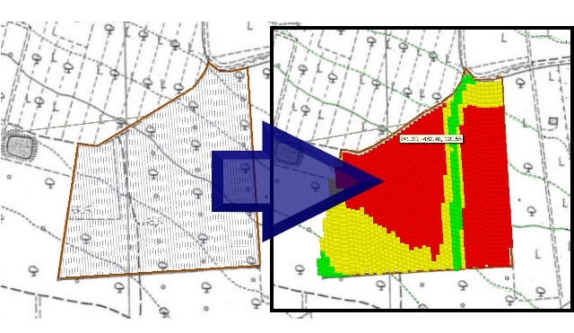
On following table it shows the consequences if it isn't considered any parameters in the calculation:
IrriPro | Other softwares | Maximum error [%] | Comments | |
Variable slope | Processing 3D model of the ground for a variable slope, point by point, section by section, pipe by pipe | Inserting a constant slope for all parts of the system | 40% for the value of uniformity50% for the minimum pressure | The error varies according to the order they are presented with the change of slope |
Variables speed | Calculated as a variable in every point | Set as a constant value | - | In general, the water speed varies in lateral pipes between 5m/s and 0 m/s |
Costant Head losses | Calculated assuming Variables the flow rates of each part of pipe and the outgoing flow from each emitter (rigorous formulation of the equation of motion and continuity) | Calculated by taking the equivalent discharge transiting the entire length of the pipeline | 30% of the total head losses | The evolution of pressure due to continuous losses, calculated as the equivalent discharge of service along the pipe, has a constant slope and differently by reality. The calculation of uniformity in this case is not reliable |
Local head losses | Considered using a rigorous formulation depending on the size of the emitter | Not considered or imposed as a constant proportion of the pressure | 50% of the total head losses | The local head losses (due to the presence of emitters) include up to 50% of the total head losses |
Integral calculus of the system | Integral calculus of all processed laterals considering their mutual interaction between each element | Calculation on a single chosen lateral | - | The reliability calculation for a single lateral (the result is then extended to the whole system) depends on the choice of the lateral and the size of the system |
Temperature | Modifiable | Not modifiable | 7-10% of the total pressures | Temperature affects the viscosity and density of water |
In conclusion, the error committed not considering any or all of the components of the calculation may become significant. In other words, a simple calculation gives no guarantee to the success of a project.
 In IrriPro the elements of a
  Thanks to IrriPro's innovative technology, which has achieved some